A Deep Dive into SciPy’s ndimage Module — by Codes With Pankaj
SciPy is a powerful library in the Python ecosystem, primarily used for scientific and technical computing. One of its essential submodules, ndimage, provides functions for multidimensional image processing. In this blog post, we will explore the ndimage module and provide practical examples of how it can be used in various image processing tasks.
Install a headless version of OpenCV :
pip install opencv-python-headlessImporting the ndimage Module
Before we dive into examples, let’s start by importing the necessary libraries:
import numpy as np
from scipy import ndimage
import matplotlib.pyplot as plt
We import NumPy for array manipulation, SciPy’s ndimage for image processing, and Matplotlib for visualization.
1. Loading and Displaying the Image:
This example loads and displays your image.
import numpy as np
from scipy import ndimage
import matplotlib.pyplot as plt
from PIL import Image

# Load your image
image_path = "p4n.jpg"
image = Image.open(image_path)
image = np.array(image)

# Display the image
plt.imshow(image)
plt.title('Your Image: p4n.jpg')
plt.axis('off')
plt.show()
2. Gaussian Filter:
This example applies a Gaussian filter to your image to create a blurred version.
# Apply a Gaussian filter
blurred_image = ndimage.gaussian_filter(image, sigma=2)

# Display the original and blurred images
plt.figure(figsize=(12, 5))
plt.subplot(121)
plt.imshow(image)
plt.title('Original Image')
plt.axis('off')
plt.subplot(122)
plt.imshow(blurred_image)
plt.title('Blurred Image')
plt.axis('off')
plt.show()
3. Sobel Filter:
This example applies a Sobel filter to your image for edge detection.
# Apply a Sobel filter for edge detection
sobel_image = ndimage.sobel(image)

# Display the original and Sobel-filtered images
plt.figure(figsize=(12, 5))
plt.subplot(121)
plt.imshow(image, cmap='gray')
plt.title('Original Image')
plt.axis('off')
plt.subplot(122)
plt.imshow(np.abs(sobel_image), cmap='gray')
plt.title('Sobel Filtered Image')
plt.axis('off')
plt.show()
4. Image Rotation:
This example rotates your image by a specified angle (e.g., 45 degrees).
from scipy.ndimage import rotate

# Rotate the image
rotated_image = rotate(image, angle=45, reshape=False, mode='constant', cval=255)

# Display the original and rotated images
plt.figure(figsize=(12, 5))
plt.subplot(121)
plt.imshow(image)
plt.title('Original Image')
plt.axis('off')
plt.subplot(122)
plt.imshow(rotated_image)
plt.title('Rotated Image (45 degrees)')
plt.axis('off')
plt.show()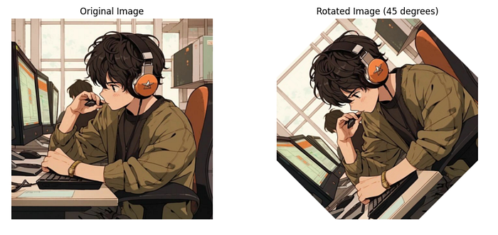
5. Image Histogram:
This example calculates and plots the histogram of pixel intensities in your image.
# Calculate the histogram
hist, bins = np.histogram(image, bins=256, range=(0, 256))

# Plot the histogram
plt.figure(figsize=(10, 5))
plt.plot(hist, color='black')
plt.title('Image Histogram')
plt.xlabel('Pixel Value')
plt.ylabel('Frequency')
plt.grid()
plt.show()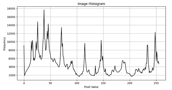
6. Image Thresholding:
This example applies a threshold to your image to convert it into a binary image.
# Apply thresholding to convert the image to binary
import cv2
import numpy as np
from scipy import ndimage
import matplotlib.pyplot as plt

# Load an image from a file
image = cv2.imread('p4n.jpg', cv2.IMREAD_GRAYSCALE)

# Apply a Gaussian filter
image_filtered = ndimage.gaussian_filter(image, sigma=5)

# Apply thresholding to convert the image to binary
threshold_value = 120
binary_image = (image_filtered > threshold_value).astype(np.uint8)

# Display the original and thresholded images
plt.figure(figsize=(12, 5))
plt.subplot(121)
plt.imshow(image, cmap='gray')
plt.title('Original Image')
plt.axis('off')
plt.subplot(122)
plt.imshow(binary_image, cmap='gray')
plt.title('Thresholded Image')
plt.axis('off')
plt.show()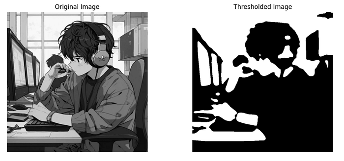
7. Image Inversion:
This example inverts the colors of your image.
# Invert the image
inverted_image = 255 - image
# Display the original and inverted images
plt.figure(figsize=(12, 5))
plt.subplot(121)
plt.imshow(image)
plt.title('Original Image')
plt.axis('off')
plt.subplot(122)
plt.imshow(inverted_image)
plt.title('Inverted Image')
plt.axis('off')
plt.show()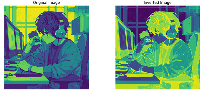
8. Zooming In and Cropping:
This example zooms in on a specific region of your image and crops it.
# Define the region to crop (coordinates of the top-left and bottom-right corners)
top, left = 100, 200
bottom, right = 300, 400
cropped_image = image[top:bottom, left:right]
# Display the original and cropped images
plt.figure(figsize=(12, 5))
plt.subplot(121)
plt.imshow(image)
plt.title('Original Image')
plt.axis('off')
plt.subplot(122)
plt.imshow(cropped_image)
plt.title('Cropped Image')
plt.axis('off')
plt.show()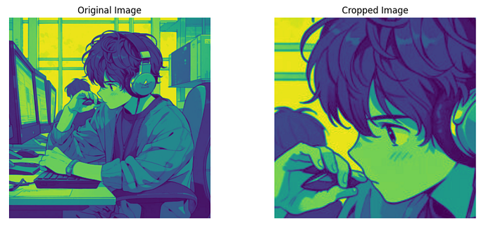
9. Color Slicing:
This example slices and displays the red, green, and blue channels of your image separately.
import cv2
import numpy as np
import matplotlib.pyplot as plt

# Load a grayscale image
image = cv2.imread('p4n.jpg', cv2.IMREAD_GRAYSCALE)

# Create pseudo-color channels by replicating the grayscale image
red_channel = image
green_channel = image
blue_channel = image

# Display the individual color channels
plt.figure(figsize=(12, 4))
plt.subplot(131)
plt.imshow(red_channel, cmap='Reds')
plt.title('Red Channel')
plt.axis('off')
plt.subplot(132)
plt.imshow(green_channel, cmap='Greens')
plt.title('Green Channel')
plt.axis('off')
plt.subplot(133)
plt.imshow(blue_channel, cmap='Blues')
plt.title('Blue Channel')
plt.axis('off')
plt.show()
10. Erosion and Dilation (Morphological Operations):
This example demonstrates erosion and dilation, which are morphological operations applied to binary images.
# Convert the image to a binary image (thresholding)
threshold_value = 128
binary_image = image > threshold_value
# Apply erosion and dilation
eroded_image = ndimage.binary_erosion(binary_image)
dilated_image = ndimage.binary_dilation(binary_image)
# Display the original binary image, eroded, and dilated images
plt.figure(figsize=(15, 5))
plt.subplot(131)
plt.imshow(binary_image, cmap='gray')
plt.title('Binary Image')
plt.axis('off')
plt.subplot(132)
plt.imshow(eroded_image, cmap='gray')
plt.title('Eroded Image')
plt.axis('off')
plt.subplot(133)
plt.imshow(dilated_image, cmap='gray')
plt.title('Dilated Image')
plt.axis('off')
plt.show()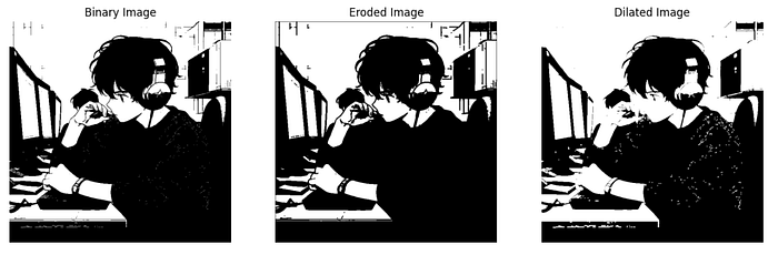
11. Labeling Connected Components:
This example labels and identifies connected components in a binary image.
# Convert the image to a binary image (thresholding)
threshold_value = 128
binary_image = image > threshold_value
# Label connected components
labeled_image, num_features = ndimage.label(binary_image)
# Display the labeled image
plt.figure(figsize=(10, 5))
plt.subplot(121)
plt.imshow(binary_image, cmap='gray')
plt.title('Binary Image')
plt.axis('off')
plt.subplot(122)
plt.imshow(labeled_image, cmap='tab20b')
plt.title(f'Connected Components (Num: {num_features})')
plt.axis('off')
plt.show()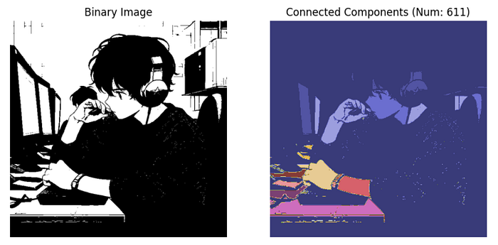
12. Distance Transform:
This example calculates the distance transform of a binary image.
# Convert the image to a binary image (thresholding)
threshold_value = 128
binary_image = image > threshold_value
# Calculate the distance transform
distance_transform = ndimage.distance_transform_edt(binary_image)
# Display the distance transform
plt.figure(figsize=(12, 5))
plt.subplot(121)
plt.imshow(binary_image, cmap='gray')
plt.title('Binary Image')
plt.axis('off')
plt.subplot(122)
plt.imshow(distance_transform, cmap='viridis')
plt.title('Distance Transform')
plt.axis('off')
plt.show()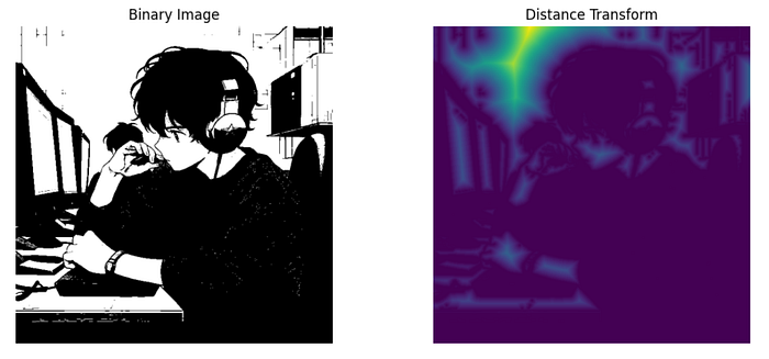
13. Morphological Gradient:
This example computes the morphological gradient of a binary image, which highlights the boundaries of objects.
# Convert the image to a binary image (thresholding)
import numpy as np
from scipy import ndimage
import matplotlib.pyplot as plt

# Assuming you have loaded your image into the 'image' variable

# Convert the image to a binary image (thresholding)
threshold_value = 128
binary_image = image > threshold_value

# Define the size parameter for morphological gradient
size = (3, 3)  # You can adjust this to change the neighborhood size

# Compute the morphological gradient
morphological_gradient = binary_image ^ ndimage.grey_erosion(binary_image, size=size)

# Display the binary image and its morphological gradient
plt.figure(figsize=(12, 5))
plt.subplot(121)
plt.imshow(binary_image, cmap='gray')
plt.title('Binary Image')
plt.axis('off')
plt.subplot(122)
plt.imshow(morphological_gradient, cmap='gray')
plt.title('Morphological Gradient')
plt.axis('off')
plt.show()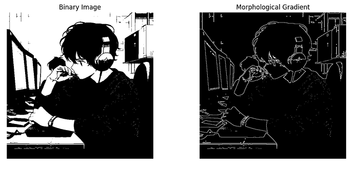
14. Edge Enhancement with Convolution:
This example enhances edges in your image using a convolution filter.
# Define an edge enhancement kernel
edge_kernel = np.array([[0, 1, 0],
                        [1, -4, 1],
                        [0, 1, 0]])
# Apply convolution to enhance edges
edge_enhanced_image = ndimage.convolve(image, edge_kernel)
# Display the original image and the edge-enhanced image
plt.figure(figsize=(12, 5))
plt.subplot(121)
plt.imshow(image, cmap='gray')
plt.title('Original Image')
plt.axis('off')
plt.subplot(122)
plt.imshow(edge_enhanced_image, cmap='gray')
plt.title('Edge-Enhanced Image')
plt.axis('off')
plt.show()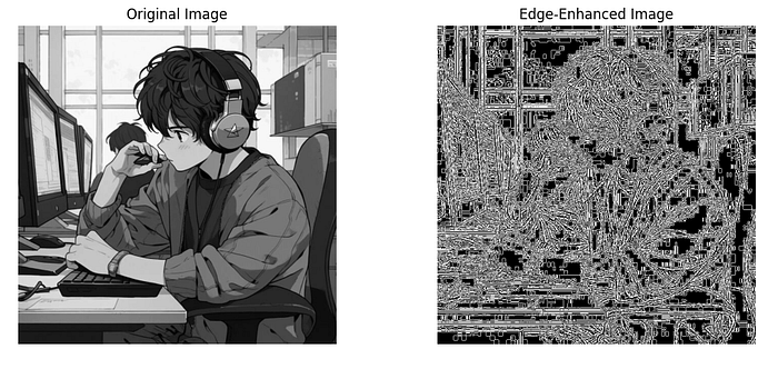
15. Hough Transform for Line Detection:
This example applies the Hough transform to detect lines in your image.
pip install scikit-imagefrom skimage.transform import hough_line, hough_line_peaks
# Convert the image to a grayscale image
from skimage import io, color
# Load the color image
image = io.imread('p4n.jpg')
# Convert the color image to grayscale
gray_image = color.rgb2gray(image)
gray_image = np.mean(image, axis=2)
# Perform Hough transform for line detection
h, theta, d = hough_line(gray_image)
# Extract line parameters from Hough space
peaks = hough_line_peaks(h, theta, d, threshold=0.5 * h.max())
# Plot the detected lines
fig, ax = plt.subplots(figsize=(8, 5))
ax.imshow(image, cmap='gray')
for _, angle, dist in zip(*peaks):
y0 = (dist - 0 * np.cos(angle)) / np.sin(angle)
y1 = (dist - gray_image.shape[1] * np.cos(angle)) / np.sin(angle)
ax.plot((0, gray_image.shape[1]), (y0, y1), '-r')
ax.set_xlim((0, gray_image.shape[1]))
ax.set_ylim((gray_image.shape[0], 0))
ax.set_title('Hough Transform for Line Detection')
ax.axis('off')
plt.show()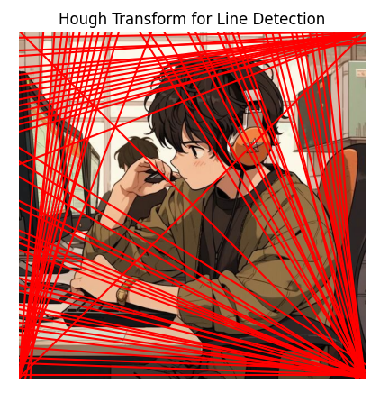
16. Image Contour Detection:
This example uses the ‘find_contours’ function to detect and plot contours in your image.
from skimage import measure
# Convert the image to grayscale
gray_image = np.mean(image, axis=2)
# Find and plot contours
contours = measure.find_contours(gray_image, 30)
plt.figure(figsize=(8, 8))
plt.imshow(gray_image, cmap='gray')
for contour in contours:
    plt.plot(contour[:, 1], contour[:, 0], linewidth=2)
plt.title('Contour Detection')
plt.axis('off')
plt.show()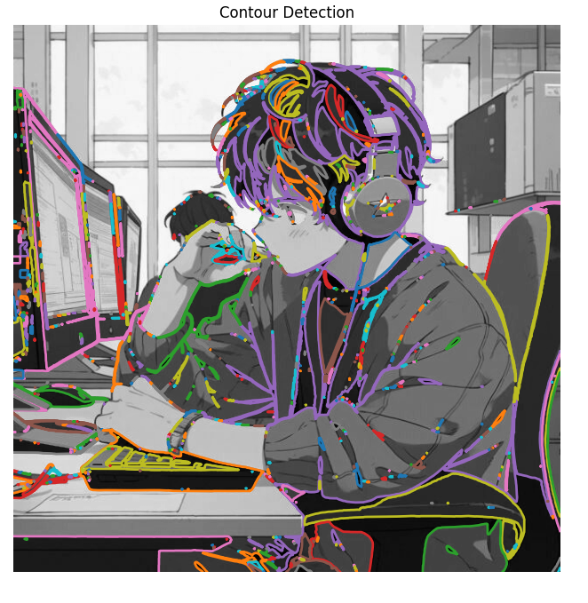
17. Histogram Equalization:
This example performs histogram equalization to enhance the contrast of your image.
from skimage import exposure
# Convert the image to grayscale
gray_image = np.mean(image, axis=2)
# Perform histogram equalization
equalized_image = exposure.equalize_hist(gray_image)
# Display the original and equalized images
plt.figure(figsize=(12, 5))
plt.subplot(121)
plt.imshow(gray_image, cmap='gray')
plt.title('Original Image')
plt.axis('off')
plt.subplot(122)
plt.imshow(equalized_image, cmap='gray')
plt.title('Equalized Image')
plt.axis('off')
plt.show()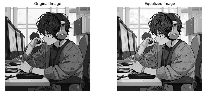
18. Image Deconvolution:
This example demonstrates deconvolution to recover a blurred image.
import numpy as np
import matplotlib.pyplot as plt
from scipy.signal import convolve2d
from scipy.signal import fftconvolve
from skimage import color, io

# Load an example image (replace 'image.jpg' with your image file)
image = io.imread('p4n.jpg')

# Convert the image to grayscale
gray_image = color.rgb2gray(image)

# Create a blurred version of the image
blur_kernel = np.array([[1, 4, 6, 4, 1],
                        [4, 16, 24, 16, 4],
                        [6, 24, 36, 24, 6],
                        [4, 16, 24, 16, 4],
                        [1, 4, 6, 4, 1]]) / 256.0

blurred_image = convolve2d(gray_image, blur_kernel, mode='same', boundary='wrap', fillvalue=255)

# Deconvolve to recover the original image
recovered_image = fftconvolve(blurred_image, np.flipud(np.fliplr(blur_kernel)), mode='same')
recovered_image = np.clip(recovered_image, 0, 1)  # Clip values to the [0, 1] range

# Display the original, blurred, and recovered images
plt.figure(figsize=(15, 5))
plt.subplot(131)
plt.imshow(gray_image, cmap='gray')
plt.title('Original Image')
plt.axis('off')
plt.subplot(132)
plt.imshow(blurred_image, cmap='gray')
plt.title('Blurred Image')
plt.axis('off')
plt.subplot(133)
plt.imshow(recovered_image, cmap='gray')
plt.title('Recovered Image')
plt.axis('off')
plt.show()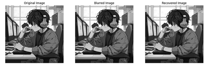
19. Object Measurement and Labeling:
This example measures the properties of objects in a binary image and labels them.
# Convert the image to a binary image (thresholding)
import numpy as np
import matplotlib.pyplot as plt
from scipy import ndimage as ndi
from skimage import io, color, measure

# Load an example binary image (replace 'binary_image.jpg' with your image file)
image = io.imread('p4n.jpg')

# Ensure that the image is 2D (if it's 3D, convert it to 2D)
if len(image.shape) == 3:
    image = color.rgb2gray(image)

# Label connected components
labeled_image, num_features = ndi.label(image)

# Calculate properties of objects
object_props = measure.regionprops(labeled_image)

# Display the original binary image and labeled objects
plt.figure(figsize=(12, 5))
plt.subplot(121)
plt.imshow(image, cmap='gray')
plt.title('Binary Image')
plt.axis('off')
plt.subplot(122)
plt.imshow(labeled_image, cmap='tab20b')
plt.title(f'Labeled Objects (Num: {num_features})')
plt.axis('off')

# Print properties of each object
for i, props in enumerate(object_props):
    print(f'Object {i + 1}: Area={props.area}, Perimeter={props.perimeter}, Centroid={props.centroid}')

plt.show()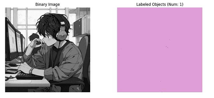
20. Image Denoising with Median Filter:
This example applies a median filter to denoise your image.
from scipy.ndimage import median_filter

# Add random noise to the image
noisy_image = image + 50 * np.random.normal(size=image.shape).astype(np.uint8)

# Apply a median filter to denoise
selem = np.ones((3, 3), dtype=np.uint8)  # Define the footprint (structuring element)
denoised_image = median_filter(noisy_image, footprint=selem)

# Display the noisy and denoised images
plt.figure(figsize=(12, 5))
plt.subplot(121)
plt.imshow(noisy_image, cmap='gray')
plt.title('Noisy Image')
plt.axis('off')
plt.subplot(122)
plt.imshow(denoised_image, cmap='gray')
plt.title('Denoised Image')
plt.axis('off')
plt.show()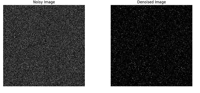
Conclusion
The SciPy ndimage module is a powerful tool for image processing tasks in Python. It offers a wide range of functions for image filtering, morphology, measurements, and more. In this blog post, we’ve only scratched the surface of what you can do with this module. By exploring the documentation and experimenting with different functions, you can perform more advanced image processing tasks.
Whether you’re working on computer vision projects, medical imaging, or any application that involves image analysis, the SciPy ndimage module is a valuable asset in your toolkit. It provides efficient and flexible solutions for a wide range of image processing needs.