Unlocking the Power of SciPy: A Comprehensive Beginner’s Guide

Cluster analysis, a fundamental technique in the field of data analysis and machine learning, aims to group similar data points together while keeping dissimilar points apart. This technique is particularly useful for finding patterns in data, identifying anomalies, and making data-driven decisions. SciPy, a scientific library in Python, offers a powerful suite of tools for cluster analysis. In this blog post, we’ll explore the basics of cluster analysis using SciPy with illustrative examples.

What is Cluster Analysis?

Cluster analysis, also known as clustering or unsupervised learning, is a method that partitions data into groups or clusters. The primary objective is to maximize the similarity within each group and minimize the similarity between different groups. It’s a versatile tool with applications in various fields, such as marketing, biology, and image processing.

SciPy provides a range of clustering algorithms that can help you identify meaningful patterns in your data. Let’s delve into some of the commonly used techniques.

Central Clustering

Central clustering, also known as partitional clustering, aims to partition the data into a predefined number of clusters, where each data point belongs to exactly one cluster. One of the most popular partitional clustering methods is K-means. Let’s dive into an example using SciPy.

K-Means Clustering

K-means clustering is an iterative algorithm that assigns data points to clusters, with the goal of minimizing the within-cluster variance. SciPy does not have a built-in K-means implementation, so we’ll use the scikit-learn library to perform K-means clustering. Here's an example:

import numpy as np
import matplotlib.pyplot as plt
from sklearn.cluster import KMeans
# Generate some sample data
data = np.array([[2, 3], [3, 3], [3, 4], [5, 4], [5, 5], [6, 5]])
# Create a K-means model with 2 clusters
kmeans = KMeans(n_clusters=2)
kmeans.fit(data)
# Get cluster labels for each data point
labels = kmeans.labels_
# Plot the data points with different colors for each cluster
plt.scatter(data[:, 0], data[:, 1], c=labels, cmap='viridis')
plt.xlabel('Feature 1')
plt.ylabel('Feature 2')
plt.title('K-Means Clustering')
plt.show()

In this example, we have used K-means to separate data points into two clusters. The algorithm assigns each data point to the cluster with the nearest centroid, creating a clear separation of the data.

Hierarchical Clustering

Hierarchical clustering, as the name suggests, builds a hierarchy of clusters. It doesn’t require specifying the number of clusters in advance and is often represented as a dendrogram. Let’s explore hierarchical clustering using SciPy.

Hierarchical Clustering

Hierarchical clustering is available in SciPy through the scipy.cluster.hierarchy module. Here's an example using the Ward linkage method:

import numpy as np
import matplotlib.pyplot as plt
from scipy.cluster.hierarchy import dendrogram, linkage
# Generate some sample data
data = np.array([[2, 3], [3, 3], [3, 4], [5, 4], [5, 5], [6, 5])
# Calculate linkage matrix using Ward method
Z = linkage(data, method='ward')
# Plot the dendrogram
dendrogram(Z)
plt.title('Hierarchical Clustering (Ward Linkage)')
plt.show()

The dendrogram visually represents the hierarchical structure of the clusters. You can cut the dendrogram at a certain height to obtain a specific number of clusters.

SciPy constants

SciPy is a scientific library in Python that extends the capabilities of NumPy by providing additional functionality for scientific and engineering applications. SciPy includes a module called scipy.constants that provides a collection of physical and mathematical constants, making it convenient for scientists and engineers to access these values. In this blog post, we'll elaborate on the scipy.constants module with some examples.

Using scipy.constants

Before using scipy.constants, you need to import the module. Here's how you can do it:

import scipy.constants as const

Once you’ve imported the module, you can access various physical and mathematical constants.

Examples of Using scipy.constants

Accessing Fundamental Constants

You can access fundamental constants like the speed of light, Planck’s constant, and the gravitational constant.

import scipy.constants as const

# Accessing Fundamental Constants
# Speed of light in meters per second (m/s)
c = const.c
# Planck's constant in joule-seconds (J·s)
h = const.Planck
# Gravitational constant in cubic meters per second squared per kilogram (m³/s²/kg)
G = const.G

print(f"Speed of light: {c} m/s")
print(f"Planck's constant: {h} J·s")
print(f"Gravitational constant: {G} m³/s²/kg")

Output :

Speed of light: 299792458.0 m/s
Planck's constant: 6.62607015e-34 J·s
Gravitational constant: 6.6743e-11 m³/s²/kg

Accessing Mathematical Constants

The scipy.constants module also provides mathematical constants, such as pi and the Euler number (e).

import scipy.constants as const

# Accessing Constants
# Value of pi (π)
pi = const.pi
# Euler's number (e)
euler = const.e

print(f"Value of pi: {pi}")
print(f"Euler's number: {euler}")

Output :

Value of pi: 3.141592653589793
Euler's number: 1.602176634e-19

Accessing Physical Constants

You can access a wide range of physical constants, including constants related to atomic and nuclear physics, electromagnetic constants, and more.

# Avogadro's number (number of atoms or molecules in a mole)
N_A = const.N_A
# Electron charge in coulombs (C)
elementary_charge = const.e
print(f"Avogadro's number: {N_A}")
print(f"Elementary charge: {elementary_charge} C")

Output :

Avogadro's number: 6.02214076e+23
Elementary charge: 1.602176634e-19 C

Conversion Factors

scipy.constants also includes conversion factors that can be handy for unit conversions. For example, you can convert from kilograms to pounds or from meters to inches:

# Conversion factor from kilograms to pounds
kg_to_pounds = const.kilogram_pound
# Conversion factor from meters to inches
m_to_inches = const.meter_inch
print(f"1 kilogram is equal to {kg_to_pounds} pounds.")
print(f"1 meter is equal to {m_to_inches} inches.")

Output :

1 kilogram is equal to 1000.0 pounds.
1 meter is equal to 0.0254 inches.

SciPy FFTpack

The SciPy library includes a module called fftpack (Fast Fourier Transform) that provides tools for performing fast Fourier transforms and related operations. The Fast Fourier Transform is a widely used mathematical technique for analyzing signals and data in the frequency domain. It allows you to transform a time-domain signal into its frequency components, making it useful in various scientific and engineering applications, including signal processing, image analysis, and spectral analysis.

Let’s explore the scipy.fftpack module with a brief overview and an example of performing a Fast Fourier Transform (FFT) in SciPy.

Overview of scipy.fftpack

The scipy.fftpack module provides several functions for working with the FFT. Some of the key functions and classes in this module include:

1. fft and ifft: Functions for 1-D Fast Fourier Transform and its inverse.
2. fftn and ifftn: Functions for n-dimensional FFT and its inverse.
3. fftfreq: Function to generate the frequency values corresponding to FFT results.
4. fftshift and ifftshift: Functions for shifting the zero-frequency component to the center of the spectrum.
5. rfft and irfft: Real-valued Fast Fourier Transform functions.

Example: Performing a 1-D FFT

Here’s a simple example of how to use the scipy.fftpack module to perform a 1-D FFT on a sample signal.

import numpy as np
from scipy.fftpack import fft, fftfreq
import matplotlib.pyplot as plt

# Sample data: A sum of two sine waves
t = np.linspace(0, 1, 1000)  # Time values from 0 to 1 second
signal = 5 * np.sin(2 * np.pi * 10 * t) + 3 * np.sin(2 * np.pi * 20 * t)

# Compute the FFT
fft_result = fft(signal)

# Generate frequency values for the FFT result
N = len(fft_result)
freq = fftfreq(N, d=t[1] - t[0])

# Plot the original signal and its FFT
plt.figure(figsize=(12, 6))

plt.subplot(2, 1, 1)
plt.plot(t, signal)
plt.title("Original Signal")
plt.xlabel("Time (s)")
plt.ylabel("Amplitude")

plt.subplot(2, 1, 2)
plt.plot(freq, np.abs(fft_result))
plt.title("FFT of the Signal")
plt.xlabel("Frequency (Hz)")
plt.ylabel("Amplitude")

plt.tight_layout()
plt.show()

In this example, we first create a sample signal by summing two sine waves with frequencies of 10 Hz and 20 Hz. We then use scipy.fftpack.fft to compute the FFT of the signal and scipy.fftpack.fftfreq to generate the corresponding frequency values. The resulting FFT plot displays the frequency components of the original signal.

The scipy.fftpack module is a powerful tool for analyzing signals and data in the frequency domain, enabling you to extract valuable information from your data, identify dominant frequencies, and perform various frequency domain operations. It's a valuable resource for engineers, scientists, and data analysts working with signal processing and spectral analysis tasks.

Multiple Integrals

Multiple integrals are a fundamental concept in calculus and mathematics, building upon the concept of single-variable integration. They extend the idea of finding the area under a curve to finding the volume, area, or higher-dimensional content of regions in multiple dimensions. Multiple integrals are used extensively in various fields, including physics, engineering, statistics, and computer science. In this blog post, we will explore the basics of multiple integrals, focusing on double integrals and triple integrals, and provide examples to illustrate their applications.

Double Integrals

A double integral is an extension of a single integral, but instead of finding the area under a curve in one dimension, it calculates the volume under a surface in two dimensions. In particular, it finds the volume of a solid that lies above a specified region in the xy-plane and below a surface defined by a function z = f(x, y).

Notation and Formula

The notation for a double integral is ∬, and it is expressed as:

∬ f(x, y) dA

Where:

• f(x, y) is the integrand, representing the function defining the surface.
• dA represents the infinitesimal area element in the xy-plane.

The formula for the double integral is:

∬ f(x, y) dA = ∫∫ f(x, y) dx dy

Example: Finding the Area

Let’s consider a simple example of finding the area of a region in the xy-plane. Suppose we want to find the area of the region R bounded by the curves y = x² and y = 2x for 0 ≤ x ≤ 1.

from scipy.integrate import dblquad

def integrand(x, y):
    return 1  # Integrate 1 over the region

result, _ = dblquad(integrand, 0, 1, lambda x: x**2, lambda x: 2*x)
print("Area:", result)

Output :

Area: 0.6666666666666666

In this example, the dblquad function integrates the constant function 1 over the specified region R, giving us the area of the region.

Triple Integrals

A triple integral extends the concept of integration to three dimensions. It calculates the volume of a region in three-dimensional space under a specified function f(x, y, z).

Notation and Formula

The notation for a triple integral is ∭, and it is expressed as:

∭ f(x, y, z) dV

Where:

• f(x, y, z) is the integrand, representing the function defining the solid.
• dV represents the infinitesimal volume element in 3D space.

The formula for the triple integral is:

∭ f(x, y, z) dV = ∫∫∫ f(x, y, z) dx dy dz

Example: Finding the Volume

Let’s consider an example of finding the volume of a region in 3D space. Suppose we want to find the volume of a solid bounded by the planes x = 0, y = 0, z = 0, x + y + z = 1.

from scipy.integrate import tplquad

def integrand(x, y, z):
    return 1  # Integrate 1 over the solid

result, _ = tplquad(integrand, 0, 1, lambda x: 0, lambda x: 1 - x, lambda x, y: 1 - x - y, lambda x, y: 1 - x - y)
print("Volume:", result)

In this example, the tplquad function integrates the constant function 1 over the specified solid, giving us the volume of the region.

SciPy Interpolation

Interpolation is a common mathematical and computational technique used to estimate data points between existing data points. It’s especially useful when you have discrete data and want to approximate values at intermediate points or when you want to smooth out noisy data. SciPy, a scientific library in Python, provides a module called scipy.interpolate that offers various interpolation methods. In this blog post, we'll explore the basics of interpolation and demonstrate how to perform it using SciPy.

Types of Interpolation

The scipy.interpolate module supports several interpolation techniques, including:

1. Linear Interpolation: This is the simplest form of interpolation. It connects two data points with a straight line. The value at any point between these data points is a linear combination of the values at those data points.
2. Polynomial Interpolation: This method uses a polynomial equation to approximate the data points. Common approaches include Lagrange interpolation and Newton interpolation.
3. Spline Interpolation: Spline interpolation involves fitting piecewise functions (typically polynomials) to the data points. Cubic splines are one of the most popular methods in this category.
4. B-spline Interpolation: B-splines are a generalization of splines that offer more flexibility in fitting curves.
5. Radial Basis Function Interpolation: Radial basis functions use a set of basis functions centered at each data point to approximate the values at other points.
6. Nearest-neighbor Interpolation: This method assigns the value of the nearest neighbor data point to the point of interest.

Example: Linear Interpolation

Let’s consider a simple example of linear interpolation using SciPy. Suppose you have a set of data points and you want to estimate values between those points.

import numpy as np
from scipy.interpolate import interp1d
import matplotlib.pyplot as plt

# Sample data points
x = np.array([0, 1, 2, 3, 4])
y = np.array([0, 2, 4, 1, 3])

# Create an interpolation function
linear_interp = interp1d(x, y, kind='linear')

# Define points where you want to interpolate
x_new = np.linspace(0, 4, num=20)
y_new = linear_interp(x_new)

# Plot the original data and the interpolated points
plt.scatter(x, y, label='Original Data', color='red')
plt.plot(x_new, y_new, label='Interpolated Data', linestyle='dotted', color='blue')
plt.xlabel('X')
plt.ylabel('Y')
plt.legend()
plt.show()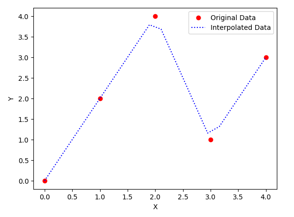

In this example, we use the interp1d function with the 'linear' kind to perform linear interpolation. We specify the x-values where we want to estimate y-values, and the function returns interpolated values. The result is a smooth curve connecting the original data points.

Finding a determinant of a square matrix

The determinant of a square matrix is a scalar value that can provide important information about the matrix, such as whether it is invertible (non-singular) or singular, and can be used in various mathematical and engineering applications. Determinants are commonly used in solving systems of linear equations and calculating eigenvalues.

To find the determinant of a square matrix, you can use several methods, depending on the size of the matrix. I’ll explain two common methods: the Laplace expansion method for smaller matrices and the LU decomposition method for larger matrices.

Method 1: Laplace Expansion (Cofactor Expansion) — For Smaller Matrices

For a 2x2 or 3x3 matrix, the Laplace expansion method is straightforward. For larger matrices, this method can become computationally intensive.

1. For a 2x2 matrix: Given a matrix:

| a  b |
| c  d |

1. The determinant is calculated as: det(A) = (a * d) - (b * c)
2. For a 3x3 matrix: Given a matrix:

| a  b  c |
| d  e  f |
| g  h  i |

The determinant is calculated as: det(A) = a(ei - fh) - b(di - fg) + c(dh - eg)

Method 2: LU Decomposition — For Larger Matrices

For larger matrices, it’s often more efficient to use LU decomposition and exploit the fact that the determinant of a product of matrices is the product of their determinants.

1. Decompose the matrix A into its lower triangular matrix (L) and upper triangular matrix (U) using LU decomposition.
2. Calculate the determinant of A using the following formula: det(A) = det(L) * det(U)
3. The determinants of L and U are relatively easy to compute as they are triangular matrices:

• The determinant of a lower triangular matrix is the product of its diagonal elements.
• The determinant of an upper triangular matrix is also the product of its diagonal elements.

Here’s a Python example using NumPy to find the determinant of a square matrix:

import numpy as np
# Create a square matrix A
A = np.array([[1, 2, 3],
              [4, 5, 6],
              [7, 8, 9]])
# Calculate the determinant using numpy.linalg.det
det_A = np.linalg.det(A)
print("Determinant of A:", det_A)

This code calculates the determinant of the 3x3 matrix A using the numpy.linalg.det function.

Keep in mind that when working with numerical computations, numerical stability is crucial, especially for large matrices with values that may lead to significant rounding errors. Numerical libraries like NumPy provide optimized and numerically stable implementations for calculating determinants.

Eigenvalues and Eigenvectors: The Basics

Eigenvalues

Eigenvalues are scalar values that represent how a linear transformation, described by a square matrix, scales a vector. For a square matrix A, an eigenvalue (λ) is a scalar that, when multiplied by a vector, results in a scaled version of the same vector:

A * v = λ * v

Where:

• A is the square matrix.
• v is the eigenvector associated with eigenvalue λ.

Eigenvectors

Eigenvectors are non-zero vectors that correspond to eigenvalues. They represent the directions along which the linear transformation only scales, without changing the direction. In other words, when a square matrix acts on an eigenvector, it merely stretches or compresses the vector, but the direction remains the same.

Finding Eigenvalues and Eigenvectors

To find eigenvalues and eigenvectors of a matrix, you need to solve the eigenvalue equation:

(A — λI) * v = 0

Where:

• A is the square matrix.
• λ is the eigenvalue.
• I is the identity matrix.
• v is the eigenvector.

Solving this equation yields both the eigenvalues and their corresponding eigenvectors.

Example: Finding Eigenvalues and Eigenvectors

Let’s consider a practical example using Python and NumPy. Suppose we have the following matrix:

A = | 3  1 |
    | 1  3 |

We want to find the eigenvalues and eigenvectors of this matrix.

import numpy as np

# Define the matrix A
A = np.array([[3, 1],
              [1, 3]])

# Calculate eigenvalues and eigenvectors
eigenvalues, eigenvectors = np.linalg.eig(A)

# Print the results
print("Eigenvalues:", eigenvalues)
print("Eigenvectors:\n", eigenvectors)

Output :

Eigenvalues: [4. 2.]
Eigenvectors:
 [[ 0.70710678 -0.70710678]
 [ 0.70710678  0.70710678]]

In this example, we use the numpy.linalg.eig function to compute the eigenvalues and eigenvectors of matrix A.

The output will provide you with the eigenvalues and their corresponding eigenvectors.

Applications of Eigenvalues and Eigenvectors

Eigenvalues and eigenvectors find application in various areas, including:

• Principal Component Analysis (PCA): Eigenvectors are used to identify the principal components of a dataset, reducing its dimensionality while retaining essential information.
• Quantum Mechanics: Eigenvalues and eigenvectors are used to describe the energy levels and wave functions of quantum systems.
• Vibration Analysis: They are applied to analyze the natural frequencies and modes of vibration in mechanical and structural systems.
• Image Compression: Eigenvalues and eigenvectors are used in image compression techniques like Singular Value Decomposition (SVD).
• Stability Analysis: In control theory, eigenvalues help determine the stability of a system.

SciPy IO (Input & Output)

The scipy.io package is a submodule of SciPy that provides a set of functions for reading and writing data in various file formats. These functions are particularly useful for working with scientific and engineering data stored in different file formats. Some of the file formats that scipy.io supports include MATLAB, IDL, Matrix Market, WAV, ARFF, NetCDF, and more. In this blog post, we'll provide an overview of how to work with these different file formats using the scipy.io package.

Reading and Writing Data in Various Formats

MATLAB Files

One of the most commonly used file formats in scientific computing is MATLAB’s .mat format. You can use scipy.io to read and write MATLAB files.

import scipy.io as sio
# Reading a MATLAB file
data = sio.loadmat('data.mat')
# Writing to a MATLAB file
sio.savemat('output.mat', {'data': data})

IDL Files

You can read and write IDL SAVE files using scipy.io.idl.

import scipy.io.idl as idl
# Reading an IDL SAVE file
data = idl.readsav('data.save')
# Writing to an IDL SAVE file
idl.savesav('output.save', data)

Matrix Market Files

Matrix Market is a common format for sparse matrices. scipy.io supports reading and writing sparse matrices in the Matrix Market format.

import scipy.io.mmio as mmio
# Reading a Matrix Market file
data = mmio.mmread('matrix.mtx')
# Writing to a Matrix Market file
mmio.mmwrite('output.mtx', data)

WAV Files

If you need to work with audio data in WAV format, you can use scipy.io.wavfile.

from scipy.io import wavfile
# Reading a WAV file
sample_rate, audio_data = wavfile.read('sound.wav')
# Writing to a WAV file
wavfile.write('output.wav', sample_rate, audio_data)

ARFF Files

ARFF (Attribute-Relation File Format) is commonly used in data mining and machine learning. You can read and write ARFF files using scipy.io.arff.

from scipy.io import arff
# Reading an ARFF file
data, meta = arff.loadarff('data.arff')
# Writing to an ARFF file
arff.dumparff('output.arff', data, meta)

NetCDF Files

NetCDF (Network Common Data Form) is a file format for storing and sharing scientific data. You can work with NetCDF files using scipy.io.netcdf.

from scipy.io import netcdf
# Reading a NetCDF file
ncfile = netcdf.netcdf_file('data.nc', 'r')
# Writing to a NetCDF file
ncfile = netcdf.netcdf_file('output.nc', 'w')

The functions provided by the scipy.io package enables us to work around with different formats of files such as:

• Matlab
• IDL
• Matrix Market
• Wave
• Arff
• Netcdf, etc.

The functions such as loadmat(), savemat() and whosmat() can load a MATLAB file, save a MATLAB file and list variables in a MATLAB file respectively.

SciPy Ndimage

Basic manipulations − Cropping, flipping, rotating

1. Cropping an Image:

Cropping an image means selecting a specific region or portion of the image. You can use scipy.ndimage.zoom to achieve this. Here's an example:

import numpy as np
from scipy import ndimage
import matplotlib.pyplot as plt

# Create a sample image (a 2D NumPy array)
image = np.random.random((256, 256))

# Define the cropping box (coordinates of the top-left and bottom-right corners)
top_left = (50, 50)
bottom_right = (200, 200)

# Crop the image
cropped_image = image[top_left[0]:bottom_right[0], top_left[1]:bottom_right[1]]

# Display the original and cropped images
plt.figure(figsize=(8, 4))
plt.subplot(121)
plt.imshow(image, cmap='gray')
plt.title('Original Image')
plt.subplot(122)
plt.imshow(cropped_image, cmap='gray')
plt.title('Cropped Image')
plt.show()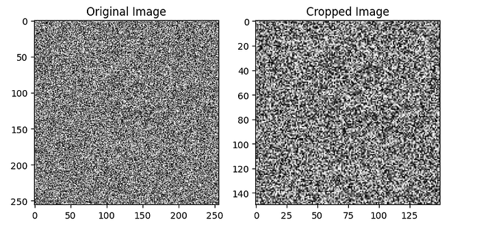

2. Flipping an Image:

You can use scipy.ndimage.flip to flip an image horizontally, vertically, or in both directions. Here's an example of flipping an image horizontally:

import numpy as np
import matplotlib.pyplot as plt

# Create a sample image (a 2D NumPy array)
image = np.random.random((256, 256))

# Flip the image horizontally
flipped_image = np.fliplr(image)

# Display the original and flipped images
plt.figure(figsize=(8, 4))
plt.subplot(121)
plt.imshow(image, cmap='gray')
plt.title('Original Image')
plt.subplot(122)
plt.imshow(flipped_image, cmap='gray')
plt.title('Horizontally Flipped Image')
plt.show()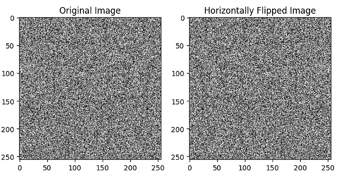

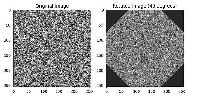
3. Rotating an Image:

To rotate an image, you can use scipy.ndimage.rotate. Here's an example of rotating an image by 45 degrees:

Download Codes